In the previous article, I covered the first building block of Elliptic Curve Cryptography (ECC): finite fields and their mathematical operations. In this article I will be covering the second building block: elliptic curves over real numbers.
The cryptography behind Bitcoin doesn’t actually use elliptic curves over real numbers but over finite field elements but understanding how elliptic curves work over real numbers will make it much easier to understand elliptic curves over finite fields. The beautiful thing is that all of the logic that you are about to see over real numbers translates perfectly onto finite fields, the visualisations just become a bit more abstract.
This article is a bit longer than the article on finite fields but the main reason for this is that I included a lot of visualisations and really wanted to explain every aspect of elliptic curves in an intuitive and in-depth way. I believe this to be crucial to the understanding of ECC and I think anyone with a genuine curiosity related to this topic will be able to follow along easily.
With that said, let’s dive in and look at what an elliptic curve is.
Elliptic Curves
Elliptic Curves have the form:
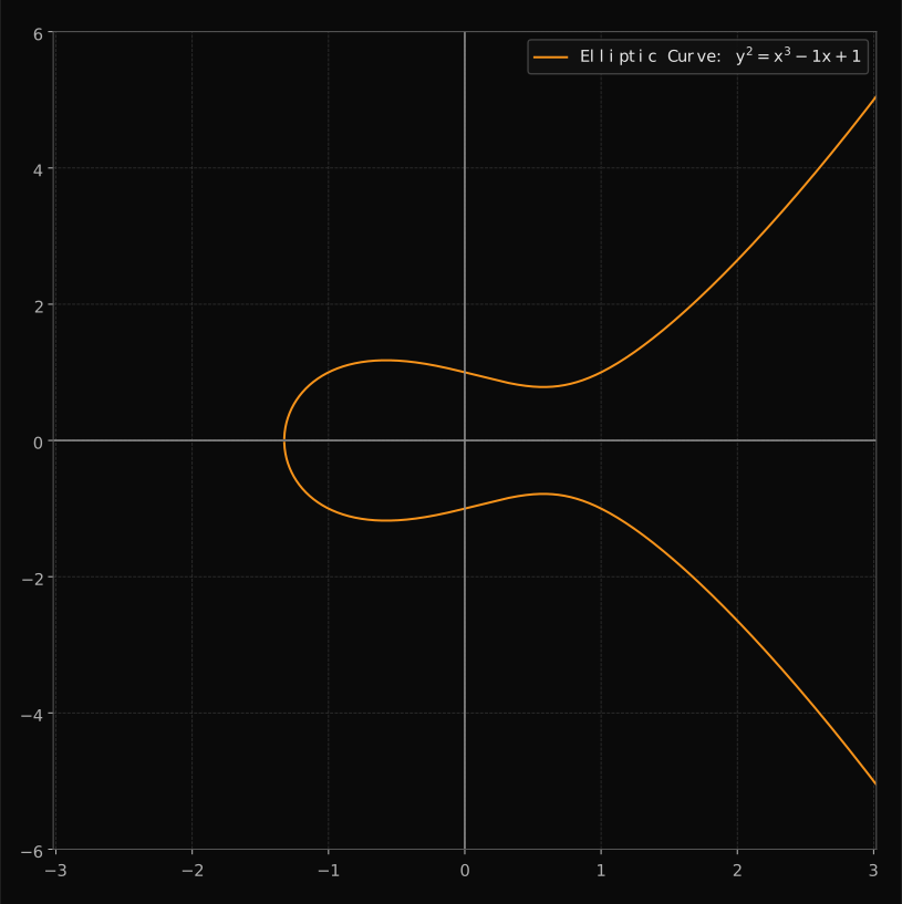
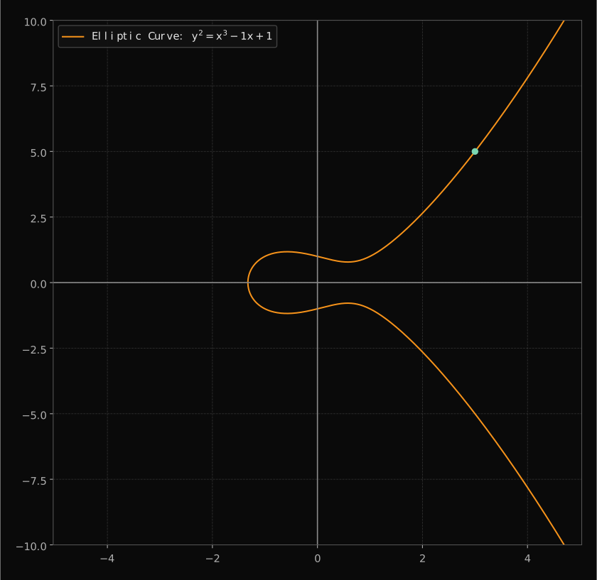
where a and b are constants that define the shape of the curve. They can be positive and negative so that, for example, for the values a = −1 and b = 1 the curve looks as follows:
 TapClick to enlarge ↗
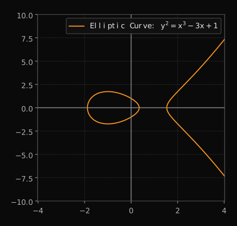
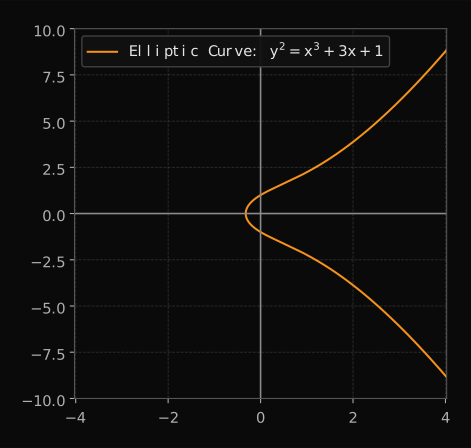
Elliptic curves over real numbers are always symmetrical about the x-axis, meaning that for most x-values there are two y-values that satisfy the equation (because of the “y2 ” on the left hand side). Different values for a and b result in different shapes. If we keep b = 1 but change a to -3 and 3, we get the following curves:
 TapClick to enlarge ↗
 TapClick to enlarge ↗
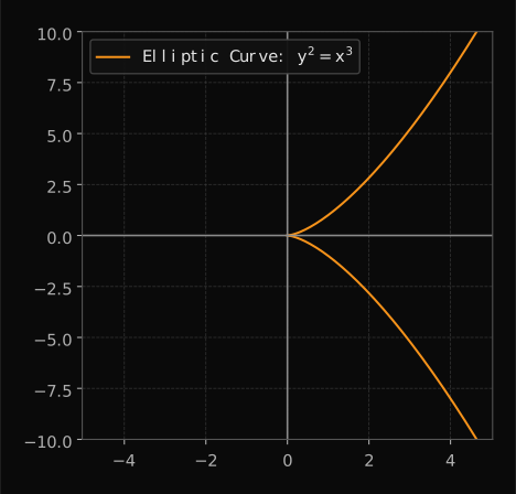
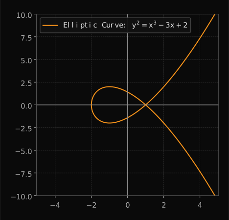
The only limitation is that 4a3 + 27b2 ≠ 0 so that we exclude singular curves, i.e. curves with cusps or self-intersections. Examples of these are the following:
 TapClick to enlarge ↗
 TapClick to enlarge ↗
Singular curves are not safe to use for cryptography because the key characteristic of non-singular elliptic curves that we rely on for elliptic curve cryptography, namely point addition, breaks down for singular curves.
Points on an Elliptic curve
A point on an elliptic curve is an (x, y) pair that satisfies y2 = x3 + ax + b for a given a and b. For the elliptic curve with a = -1 and b = 1, the point (3, 5) lies on the curve since 52 = 33 - 3 + 1:
 TapClick to enlarge ↗
Rather than thinking of elliptic curves as a continuous plot on a graph we can think of them as an infinite set of points that satisfy the elliptic curve equation. Looking at these points as a set allows us to look at them as a group, which allows us to apply the rules of a group to them. This is especially important for what’s called “point addition”. Before we get to point addition, let’s revise what groups are and what rules they follow.
Groups
A group is a set equipped with a single binary operation that satisfies four key properties: closure, associativity, identity, and invertibility. The binary operation and key properties are defined as follows:
-
Binary Operation: A binary operation on a set G is a rule that combines two elements of G to produce another element of G.
-
Closure: If a and b are in the group G, then the result of the operation a∗b must also be in G. Not that “∗” denotes the binary operation and not multiplication here.
-
Associativity: The operation must be associative, meaning (a∗b)∗c=a∗(b∗c) for all a, b, c ∈ G.
-
Identity: There must be an element e in G such that a ∗ e = e ∗ a = a for all a ∈ G. This e is called the identity element.
-
Inverse Element: For each element a in G, there must be an element b in G such that a∗b = b∗a = e, where e is the identity element. The element b is called inverse of a.
One of the amazing benefits of abstract algebra is that we can define a binary operator in any way, as long as it consistently satisfies the properties required for the structure being studied (e.g., a group, ring, field). This means that in our case we just need a definition of the binary operation that makes our elliptic curve points behave like group elements and satisy all the above properties of a group.
The binary operation that we will use (which is also the most natural and widely accepted one) is point addition.
Point Addition
Point addition is when we combine two points on the curve and get a third point, also on the curve.
To define point addition we rely on a key observation about elliptic curves:
For every elliptic curve, a line will intersect it at either three points or one point, except in a handful of special cases.
We will verify this shortly. This observation is one of the keys to understanding everything that follows. A closely related important fact is that as long as we do not pick a perfectly vertical line, if we intersect two points in an elliptic curve, then we will also intersect a third point on the elliptic curve.
The above two statements are difficult to understand without visualisations so let’s look at some real elliptic curves.
Three Intersections
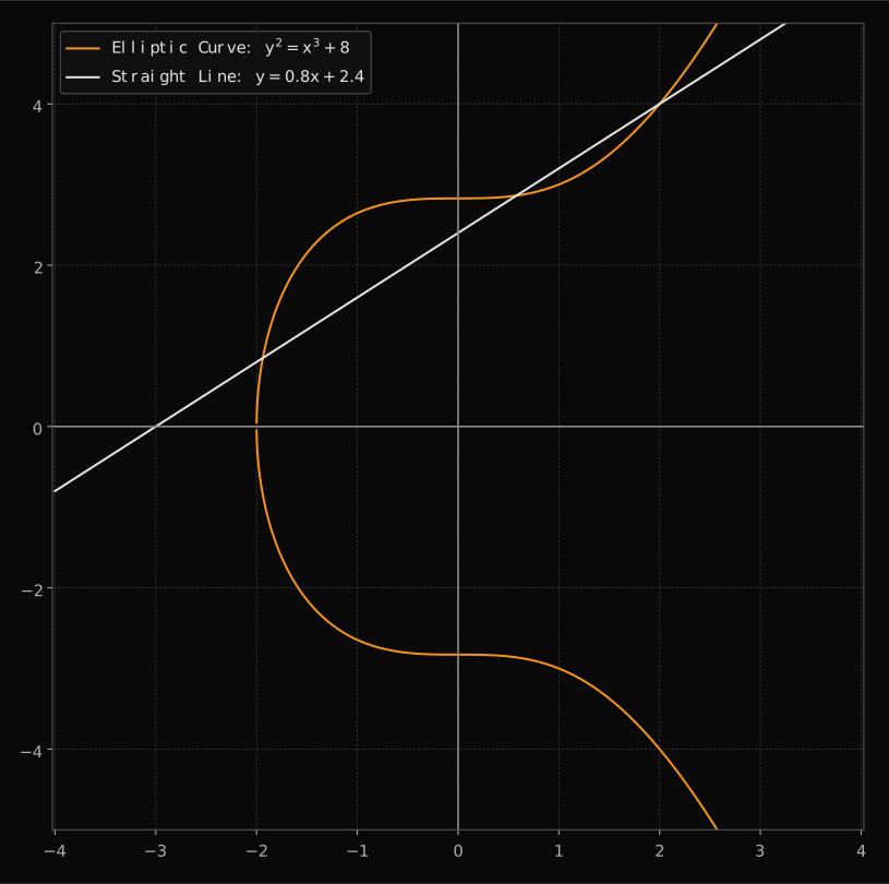
Using the set of points that satisfy the elliptic curve equation y2 = x3 + 8 as an example we can see that a straight line such as y = 0.8x + 2.4 intersects the elliptic curve at three points:
 TapClick to enlarge ↗
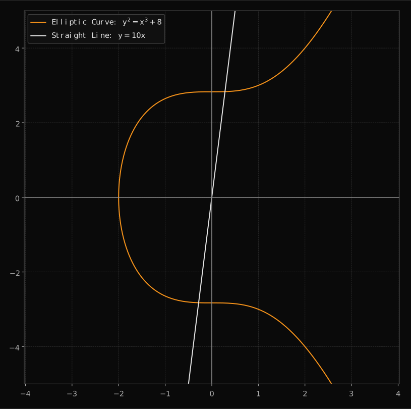
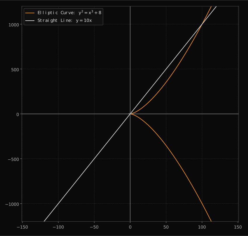
This is the case because the straight line was deliberately constructed in a way that it would intersect the elliptic curve three times within the range of the coordinate system displayed in the plot. But what about a straight line that is more vertical? Would it ever intersect the elliptic curve a third time if it intersects it at two points? Let’s look at the line y = 10x :
 TapClick to enlarge ↗
Just looking at the range of the coordinate system displayed above it looks like the white line is steeper than the orange curve and as if the two lines would not intersect a third time.
It turns out that when you zoom out far enough the two lines always eventually intersect again (as long as the white line is not perfectly vertical). The same straight line and elliptic curve eventually intersect a third time somewhere around the point (100, 1000):
 TapClick to enlarge ↗
Mathematically this is explained by taking the square root of both sides of the elliptic curve function and comparing it to the equation for the straight line:
As the value of x gets really large, the term x3 dominates the behavior of the polynomial x3 + ax + b, so that for the square root of any elliptic curve equation we get:
as x gets very large. This will eventually rise faster than any linear function y = Cx, regardless of how large C is, causing them to intersect again.
Also note that the line doesn’t have to intersect the elliptic curve at the “U-shape” part of the curve for this to be true, as you can see here:
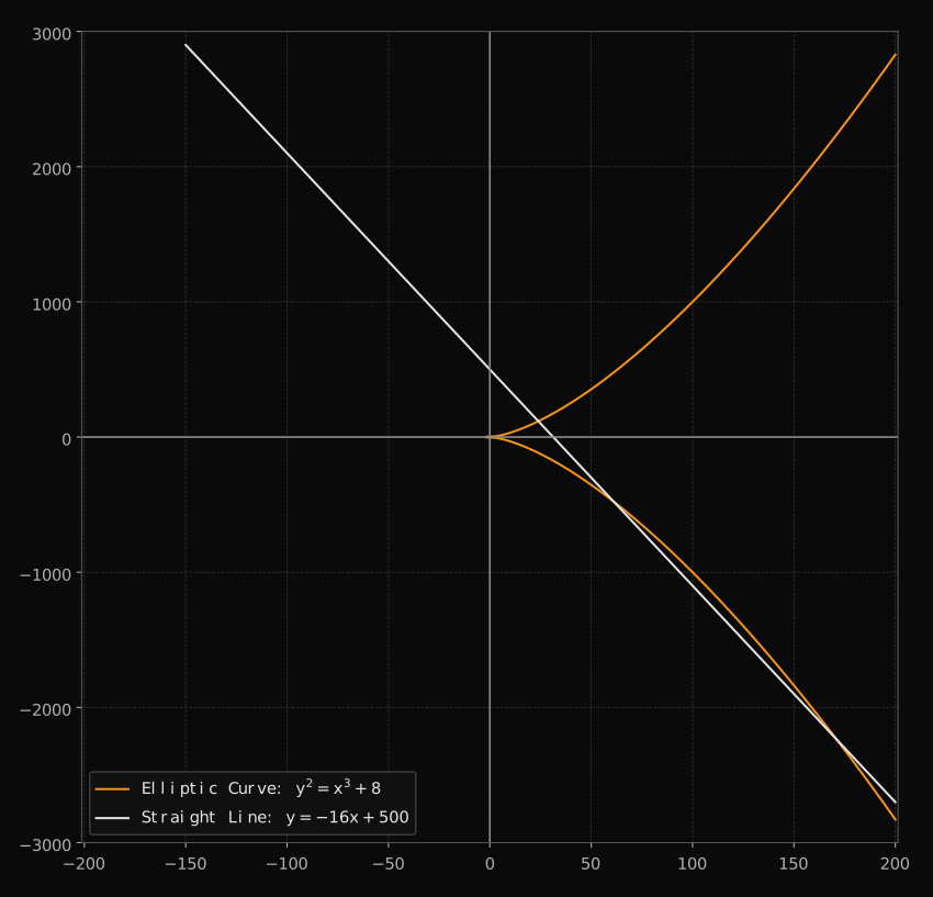 TapClick to enlarge ↗
One Intersection
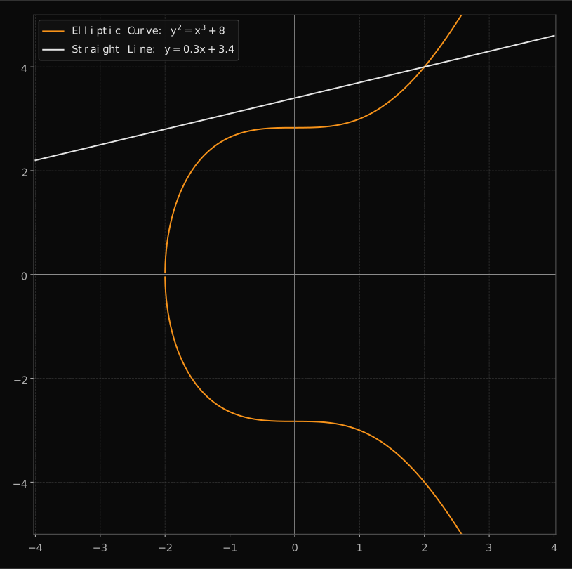
If we move the y-axis intercept up a little bit and reduce the steepness of our curve from above, we can create a scenario where the straight line intersects the elliptic curve only once:
 TapClick to enlarge ↗
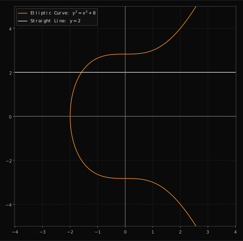
In this case, even if we zoom out further the white and orange line never intersect again. Another example for this particular curve is the perfectly horizontal line shown below:
 TapClick to enlarge ↗
The cases where we have a straight line that intersects the elliptic curve at only one point are valid for understanding elliptic curves but for the binary operation we want to define, point addition, they are irrelevant because, by definition, for point addition we need at least two points. There is a special case where we add a point to itself where intersections must be counted with multiplicity… more on this later.
Special Cases
Vertical lines
There are two special cases for vertical lines. The first is a vertical line that intersects at two points:
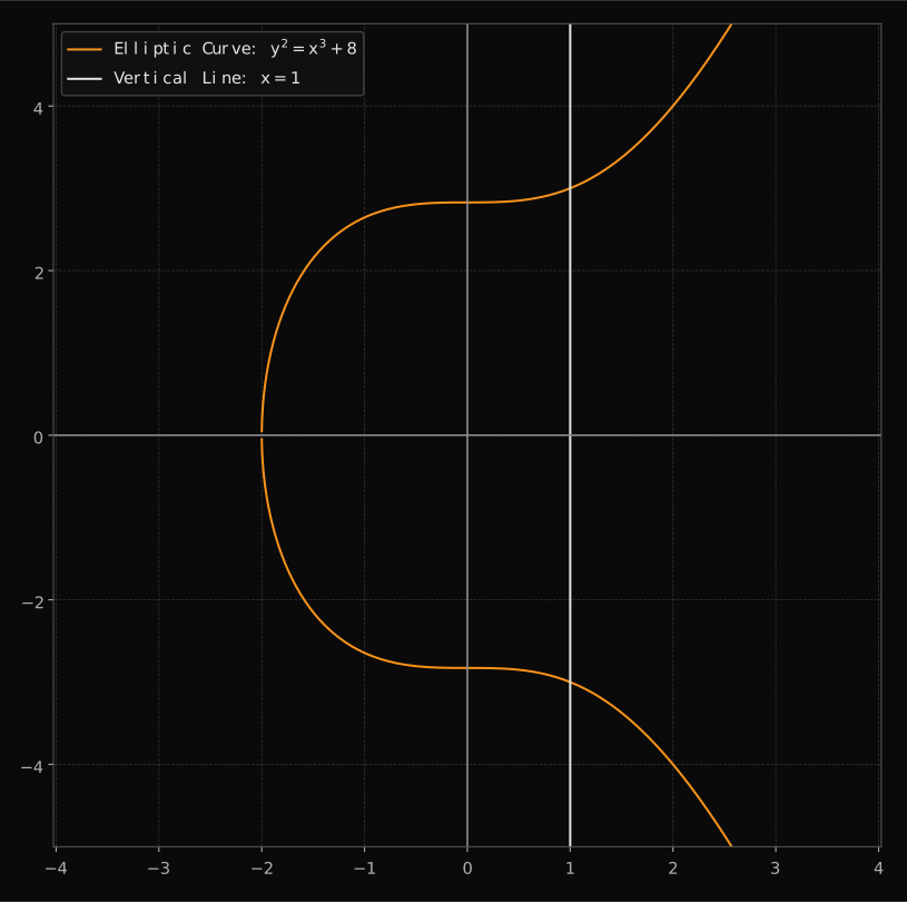 TapClick to enlarge ↗
The second is a vertical line that is tangent to the curve. In this case the vertical line will be tangent to the elliptic curve at y = 0:
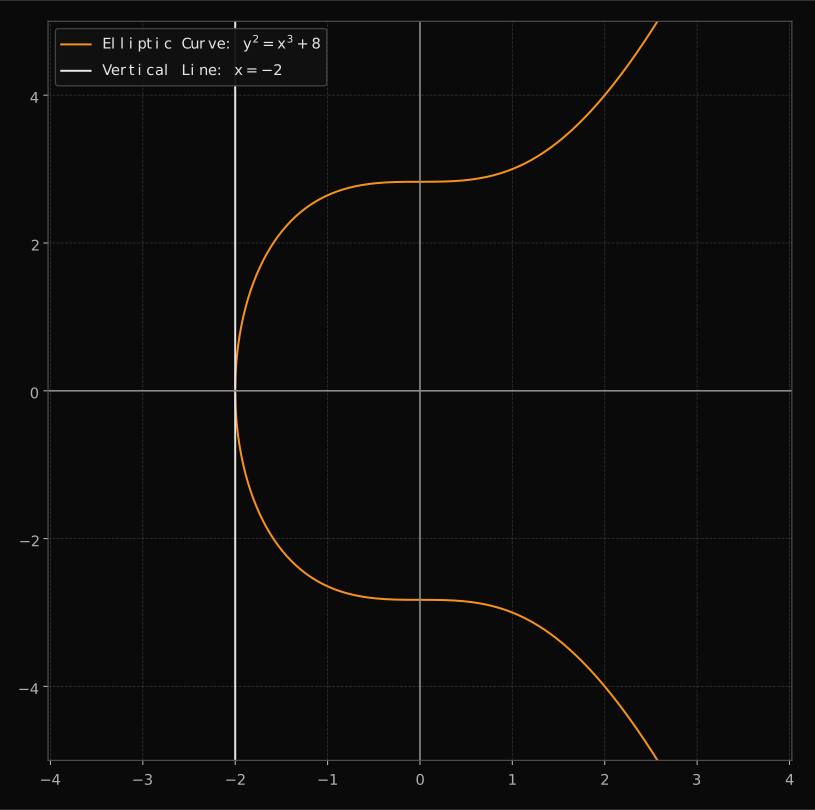 TapClick to enlarge ↗
Non-vertical tangent lines
A non-vertical tangent counts as two intersections at the point of tangency. The third intersection is usually another point, but at an inflection point all three coincide. This is due to the same logic we used to show that a non-vertical line that intersects two points on a curve must intersect at a third point. An example is the following line:
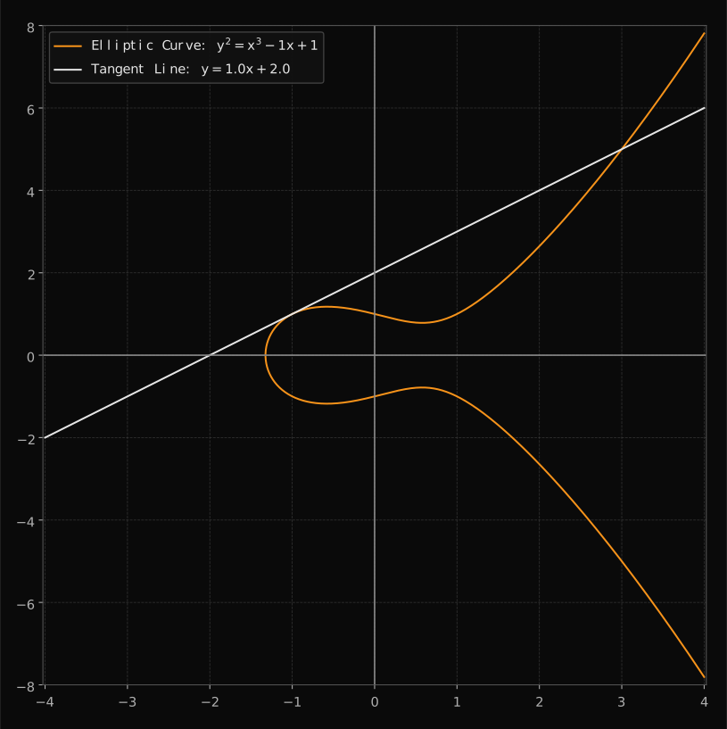 TapClick to enlarge ↗
This rule for counting the intersections of a non-vertical tangent line will be the key building block for what’s called “Scalar Multiplication”, which is just adding a point to itself a given number of times. More on this later.
Now that we have seen all of the ways in which a straight line can intersect an elliptic curve, let’s talk about how the binary operation, point addition, actually works.
How Point Addition Works
Possible scenarios
There are essentially three scenarios that we need to cover for a complete and robust implementation of point addition:
-
The two points being added are different and not on a vertical line.
-
The two points are in a vertical line or one of them is the identity element.
-
The two points are the same (adding a point to itself).
Before we look at each of these it’s important to define what the inverse of an elliptic curve point is. The inverse of an elliptic curve point is the negative of the y-value of the pair. That is, the inverse of (x, y) is (x, −y) and vice versa. Drawing a line through such points creates a perfectly vertical line:
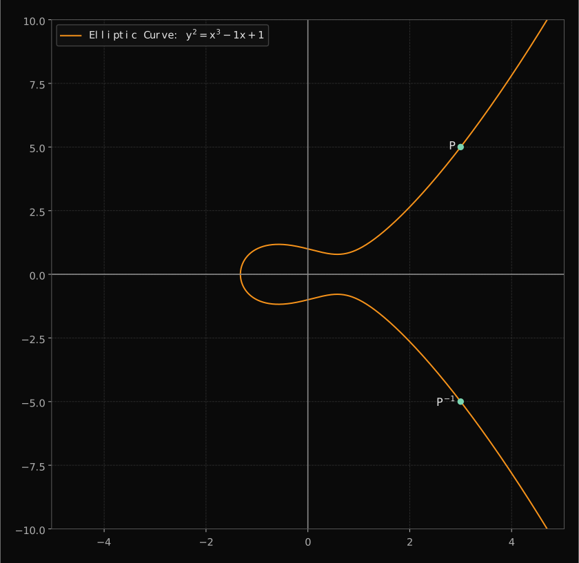 TapClick to enlarge ↗
This fact is important to know for multiple of the scenarios below.
Different Points not on a vertical line
The general logic for point addition of elliptic curve elements is the following:
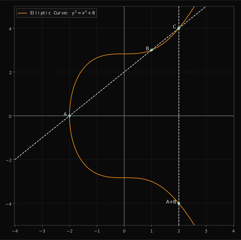
Draw a line through the two points being added together and find the point where it intersects a third time.
Reflect the resulting point over the x-axis.
Here is an example:
 TapClick to enlarge ↗
The above chart also shows that point addition is commutative, in the sense that A + B = B + A. This is because the line that intersects A and B intersects at only one other point and that point is always the same no matter the order.
The fact that we reflect the resulting point over the x-axis to get the result of point addition may seem odd but it’s required so that the definition of point addition is in line with the properties of a group and that there are no mathematical inconsistencies.
Mathematically, if we didn’t do the reflection, we would have the following set of equations that are all true:
Please note that here the “+” operator refers to point addition and not “normal” addition. If we substitue the B + C into the last equation in place of A, we get:
As we said above, the inverse of an elliptic curve point (x, y) is (x, −y), so we have a contradiction. The identity element is equal to its inverse, but so are points with y = 0, such as (−2, 0) on y2 = x3 + 8. A general point C with non-zero y is not equal to its inverse, so the proposed rule cannot define a group.
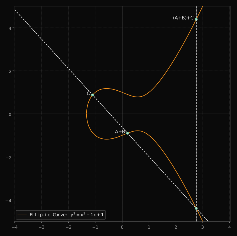
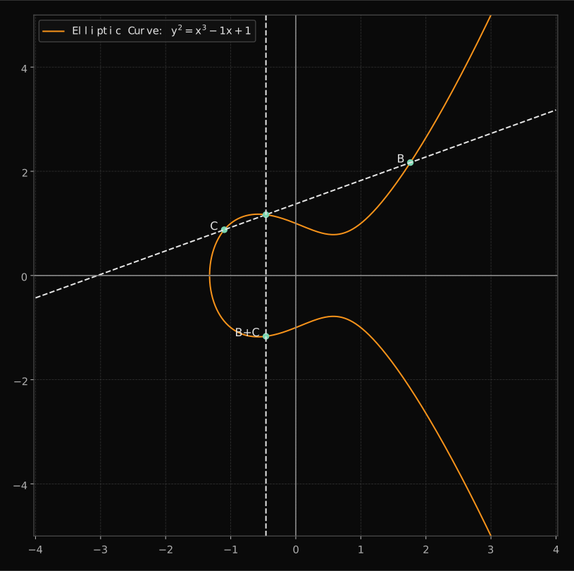
There is also a more intuitive way of understanding the importance of the reflection over the x-axis and it’s related to the condition of “Associativity” for group elements. Associativity means that (A + B) + C = A + (B + C). The below charts show visually that point addition is in fact associative. If we first add A and B:
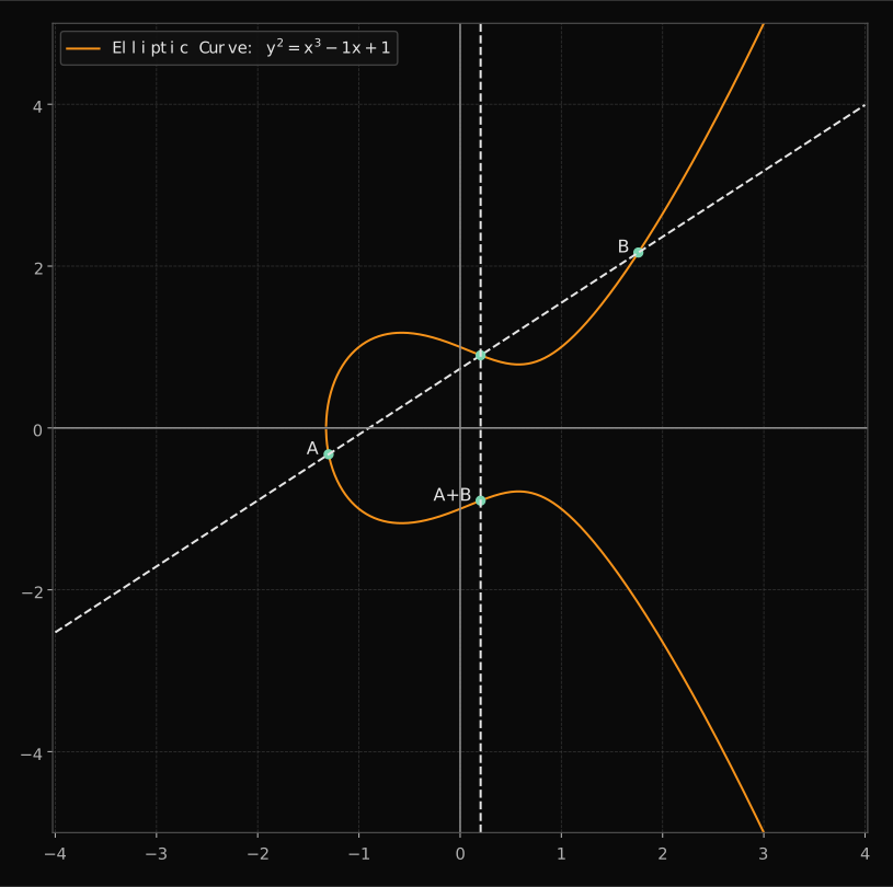 TapClick to enlarge ↗
And we then add C to (A + B), we end up at the following point:
 TapClick to enlarge ↗
Now let’s first add B and C:
 TapClick to enlarge ↗
And then add A to (B + C), to get the following point:
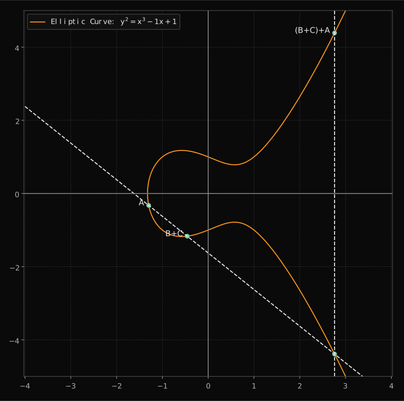 TapClick to enlarge ↗
The point (A + B) + C is indeed the same as (B + C) + A, illustrating associativity for this example when we flip over the x-axis. A general proof needs more than this diagram.
Quick pre-algebra refresher
Some of you may have wondered how exactly we calculate the point at which a line intersects for the third time so here is a quick explanation: Given two points A and B we can compute the point A + B using the slope formula from pre-algebra and then use the slope to calculate the x- and y-coordinate of A + B as follows:
Points on a vertical line or identity element
Up until now we have introduced the concept of the identity element but we haven’t actually defined it. In the properties of a group, there were two properties which relate to the identity element. To recap:
-
Identity: There must be an element e in G such that a + e = e + a = a for all a ∈ G. This e is called the identity element.
-
Inverse Element: For each element a in G, there must be an element b in G such that a + b = b + a = e, where e is the identity element. The element b is called inverse of a.
Note that the “∗” sign is replaced with “+” because “∗” was just a placeholder for a binary operation but we have since defined it as point addition, which we have denoted with “+”.
The Point at Infinity
In elliptic curve point addition, the identity element is officially called the “point at infinity”. This term is a bit confusing and it might be easier to think of this as the “point that is nowhere”. This point isn’t technically on the curve and therefore wouldn’t belong to the group but remember that in abstract algebra we can define binary operations however we like over groups arbitrarily defined, as long as the definition is consistent with the rules of a group. The group is then defined to be all the points that satisfy the elliptic curve equation and the point at infinity.
Thinking of the identity element as the “point that is nowhere” makes property 4 easy to understand because if you combine a point on the curve with nowhere then nothing changes.
Regarding property 5, we already saw that the inverse of an elliptic curve point is the negative of the y-value of the pair, as shown below:
TapClick to enlarge ↗Property 5 states that if you add the inverse of a point to the point you get the identity element. For the above points, P and P−1 this means that drawing a line between the two points, which is by definition vertical, will “intersect” again at the point at infinity, i.e. the point that is nowhere, and looks like this:
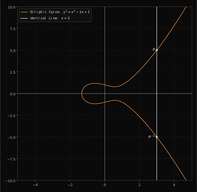 TapClick to enlarge ↗
Adding a point to itself
Adding a point to itself can be thought of as bringing two points infinitesimally close to each other until they become the same point. At that point, the slope of the line will lie tangent to the curve. Therefore, adding a point to itself can be done by simply taking the derivative at that point, getting the point where the tangent line intersects the elliptic curve again, and once again reflecting over the x-axis like so:
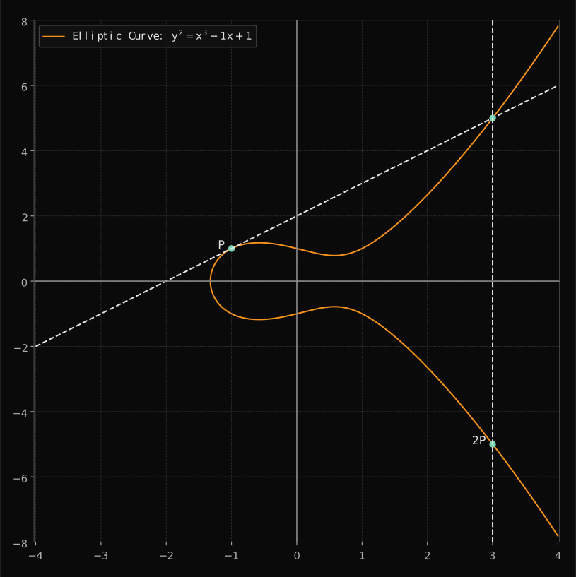 TapClick to enlarge ↗
We can also add a point to itself many more times. It’s cumbersome to visualise repeated point addition on an elliptic curve but I have created a Python class for this and we can just print the resulting coordinates as such:
from ec_rounded import EllipticCurve, ECPoint

# Initialize the elliptic curve
curve = EllipticCurve(a=-1, b=1)

# Create the starting point on the curve (P)
point = ECPoint(x=-1, y=1, curve=curve)

# Add the point to itself once (2P)
two_p = point + point
print(f'2P = {two_p.x, two_p.y}')

# Add the point to itself 7 times (8P)
eight_p = point + point + point + point + point + point + point + point
print(f'8P = {eight_p.x, eight_p.y}')
2P = (3.0, -5.0)
8P = (-1.3222773117164692, -0.10190583375353057)We can verify that the result of adding the above point, P, to itself is indeed equal to the result we saw in the visualisation, i.e. a resulting point at coordinates (3, -5). Adding P to itself 7 times results in the point with the rounded coordinates of (-1.32, -0.1).
The ability to add a point to itself on an elliptic curve enables us to do what’s called “point multiplication”, which is at the heart of how you generate public keys from private keys in Bitcoin.
Point Multiplication
Adding a point on an elliptic curve to itself a given number of times is referred to as point multiplication or scalar multiplication. The term “multiplication” is a bit misleading here because the operation is still just point addition done a given number of times.
But what if we want to do this a large number of times? If we want to do 1000⋅P for a point P on an elliptic curve, i.e. add 1000 copies of the point, do we have to do 1000 addition operations?
The answer to that is no. In fact, the number of additions is much smaller. Let’s start with a smaller example. Above, we added the point, P, with coordinates (−1, 1) on the elliptic curve y2 = x3 — x + 1 to itself 7 times to get 8P. Another way to get the same result is to add P to itself to get 2P, then add 2P to itself to get 4P and then to add 4P to itself to get 8P. In Python this looks as follows:
P = ECPoint(x=-1, y=1, curve=curve)
P_2 = P + P
P_4 = P_2 + P_2
P_8 = P_4 + P_4
print(f'8P = {P_8.x, P_8.y}')
8P = (-1.322277311716466, -0.10190583375354345)This is the same result as above but we only had to do three additions instead of 7. For 1000⋅P we could break it down into:
1000P = 512P + 256P + 128P + 64P + 32P + 8P
512P can be computed quickly because we just need to double the point 9 times. If we save all the intermediate results we also have all the other terms already and then it’s just about doing the 5 additions shown above for a total of 14 (9+5).
In CS terms, this goes from being an O(n) operation to O(log2(n)). We will talk about this in more detail when we do elliptic curves over finite fields.
The Python class implements point multiplication in this way. These real-number examples use the approximate plotting class, so rounding error accumulates; the finite-field examples use exact modular arithmetic:
P = ECPoint(1, 1, curve)

# Calculate 8P
P_8 = 8 * P
print(f'8P = {P_8.x, P_8.y}')

# Calculate 1000P
P_1000 = 1000 * P
print(f'1000P = {P_1000.x, P_1000.y}')
8P = (0.7600000000000007, -0.8239999999999981)
1000P = (9.847769504894714, 30.759954126511282)What’s the point of point addition and elliptic curves?
One of the defining features of elliptic curve cryptography lies in the unpredictability of point addition. While the mathematical formula for adding two points on the curve is straightforward, the outcome isn’t intuitively obvious.
Given two points on the curve, the result of adding them together can seem almost random. This unpredictability grows even more pronounced when we apply point multiplication, which involves adding a point to itself repeatedly. The result of this operation is computationally simple, but reversing it — determining how many times a point has been added to itself from the final result — presents a formidable challenge. This is known as the discrete logarithm problem, and it’s what makes elliptic curve cryptography so secure. For cryptographically suitable curves over finite fields, the best known generic classical attacks, such as Pollard’s rho algorithm, take roughly √n group operations, where n is the subgroup order. They are much faster than trying every multiplier, but still impractical when n is large enough. This one-way function, where the forward operation is easy but the reverse is nearly impossible, is the cornerstone of the cryptographic strength behind elliptic curves.
Now that you understand both finite fields and elliptic curves over real numbers you can move on to the next article, on elliptic curves over finite fields:
Bitcoin’s Cryptography Explained — Elliptic Curves over Finite Fields