Bitcoin’s Cryptography Explained — Elliptic Curves over Finite Fields: The Foundation of Elliptitc Curve Cryptography

In the previous two articles of this series on Bitcoin’s Cryptography, I covered finite fields and elliptic curves over real numbers. These are both fields of abstract mathematics and are absolutely vital for understanding the cryptography behind Bitcoin — Elliptic Curve Cryptography (ECC). But they are also the only two mathematical concepts that you need to understand in order to understand everything that follows and to fully understand how ECC works at a deep level.

In this article I will combine finite fields and elliptic curves, which allows us to get elliptic curves over finite fields, rather than real numbers. This is abstract math so it will be new and somewhat foreign to most readers but if you have read and understood the articles on fintie fields and elliptic curves (over real numbers) you will be able to see through the abstraction and are well equipped to understand the concepts in this article quite easily.

Elliptic Curves over Fintie Fields

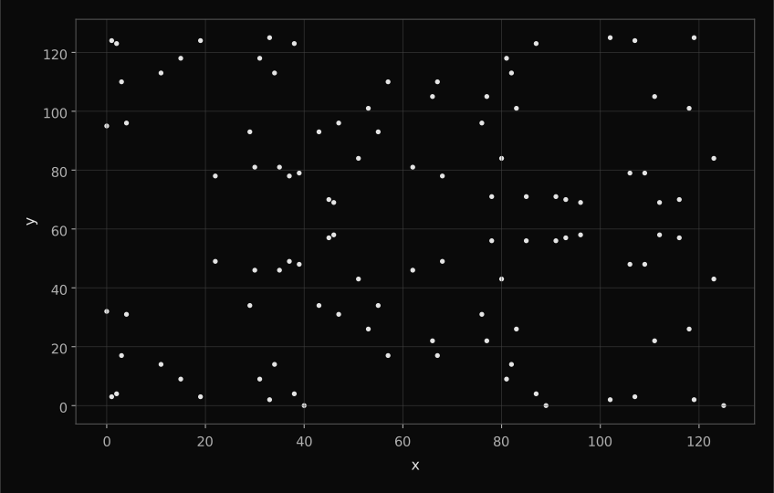
ECC relies on elliptic curves over finite fields, meaning that the coordinates of the points “on the curve” have to be elements of the fintie field over which the curve is defined. This means that they are bound to be between 0 and p-1 and have to be integer values. Because of this, we don’t obtain a smooth curve, as we do over real numbers. For example, if we plot all the points that fall on the elliptic curve y² = x³ + 8 over a finite field of order 127, we get the following plot:

Points satisfying y² = x³ + 8 modulo 127.

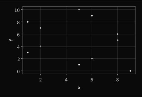
Larger prime fields generally give larger curve groups, although the number of points need not increase with every increase in the prime. Here are some examples:

Points satisfying y² = x³ + 8 modulo 11, illustrating different field sizes.

Points satisfying y² = x³ + 8 modulo 31, illustrating different field sizes.

" />

Points satisfying y² = x³ + 8 modulo 41, illustrating different field sizes.

" />

Points satisfying y² = x³ + 8 modulo 89, illustrating different field sizes.

" />

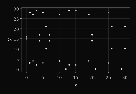
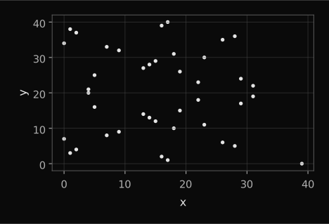
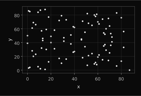
As stated above, the range of x- and y-values that lie on the “curve” are bound to be between 0 and p−1 because everything is done modulo p. Integer coordinates can be reduced modulo p into this range; arbitrary real coordinates cannot simply be wrapped into a finite field.

The symmetry remains

For non-zero y, the points come in pairs (x, y) and (x, p−y), which appear symmetric about y = p/2. Points with y = 0 are their own inverses, so they are the exception to this visual reflection rule.

Because we don’t have negative numbers in finite fields but we have modular arithmetic, the symmetric counterpart (the inverse) for any y-value is (−y) mod p, which results in the following relationships:

If y is below p/2, then the counterpart p−y is above p/2.

If y is above p/2, then the counterpart p−y is below p/2.

Connection to points on the elliptic curve over real numbers

You might be wondering whether there is a relationship between the points that we can see in the scatterplots of the elliptic curves over fintie fields and the plot that we would get if we plot the same elliptic curve over real numbers. There actually is.

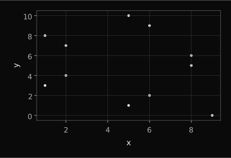
Looking at the elliptic curve y² = x³ + 8 over a finite field of order 11, we get the following plot:

Points satisfying y² = x³ + 8 modulo 11.

We can actually map some of the above points to points on the same elliptic curve over real numbers.

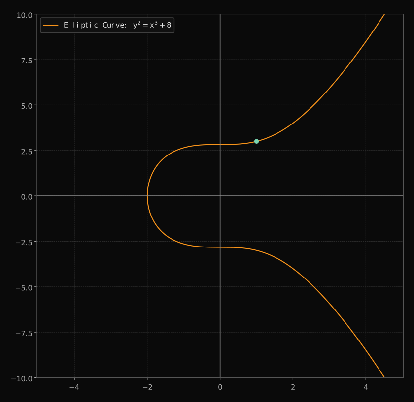
The point (1,3), for example, exists on both curves:

Integer points (1, 3), (2, 4) and their inverses on the real curve y² = x³ + 8.

The same is true for (2,4) and for the inverses of both points, as you can check in the plot above.

This is obvious for the above points because both x- and y-coordinates are less than p so that if they are points on the elliptic curve over real numbers then they would map to the same point over the fintie field of order 11 because 2 % 11 = 2 and 4 % 11 = 4, for example.

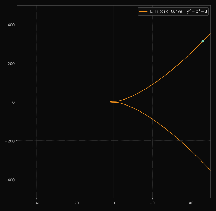
But we can even map the point (46, 312), which is on the curve over real numbers, as well as its inverse onto the finite field elements:

The integer point (46, 312) reduces to (2, 4) modulo 11.

This is because 46 is congruent to 2 and 312 is congruent to 4 modulo 11. Integer points on the real curve can be reduced modulo 11, and rational points can also be reduced when their denominators are invertible modulo 11. The reverse is not guaranteed: a finite-field point need not come from an integer point on the real curve. What carries over is the algebraic rule for point addition, with all arithmetic performed in the finite field.

The importance of that last sentence cannot be overstated because what this means is that point addition actually works over a finite field and the logic remains the same as it is over real numbers. The mathematical operations for addition and multiplication work as defined for the finite field elements, i.e. using modular arithmetic, but the logic for point addition is exactly the same and the math just works. So cool!

Point addition over a finite field

On an elliptic curve over a finite field, when you add two points, A and B, which are not the same (and don’t lie on a vertical line), then you follow the same logic used for elliptic curves over real numbers to find the result, which is:

Find the straight line that connects A and B.
Find the third point that is intersected by this line.
Reflect over the axis of symmetry (find the inverse).

Over fintie fields you don’t reflect the point from step 2 over the x-axis, because we are operating over a finite field and negative numbers aren’t allowed. In a finite field you flip over the “mirroring axis” at p/2. Because we are operating over a finite field, the straight line that connects these points wraps around at the edges, which are defined to be 0 and p−1 for both the x- and y-axis.

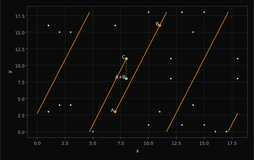
The following visualisation shows how to get the result of A + B, where A is (7, 3) and B is (11, 16), on the elliptic curve y² = x³ + 8 over a finite field of order 19:

Modulo 19, A = (7, 3) plus B = (11, 16) gives (8, 8), reflecting the third intersection (8, 11).

In the above visualisation, we first plot the line which connects the points A and B and keep drawing this out past the point B. Whenever it reaches an edge at either 0 or p-1 on the x- or y-axis it wraps around to the opposite side and continues. We do this until this line hits another point, which happens at point C with the coordinates (8, 11). As we discussed earlier, the axis of symmetry over finite fields is at p/2, which in this case is 19/2 = 9.5. Reflecting the point of third intersection over this axis gives us the final result, A + B, which is the point (8, 8).

The above example shows that the logic and the math behind point addition stays exactly the same when moving from elliptic curves over real numbers to elliptic curves over finite fields. But the key operation for ECC, and specifically for the cryptography behind Bitcoin, is point multiplication, which is adding a point to itself a given number of times.

Point Multiplication

Adding a point to itself

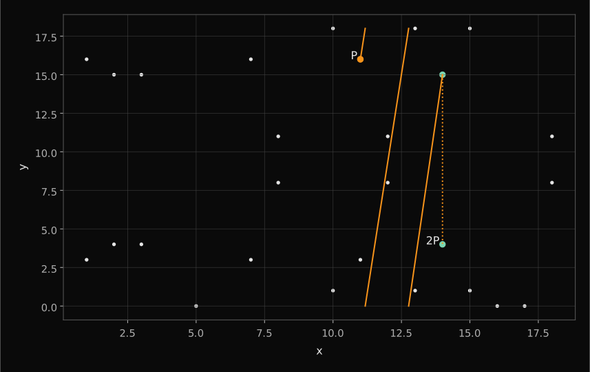
Similar to the logic for elliptic curves over real numbers, when adding a point to itself the slope of the straight line we are interested in is the slope of the tangent line at that point. The concept of a tangent line might be difficult to conceptualise here because we don’t have a continuous curve anymore but as it turns out the math for finding the slope also remains the same. Let’s use point B with coordinates (11, 16) and the same elliptic curve from above but ust rename the point to “P” for this example. When we add P to itself, it looks like this:

Doubling P = (11, 16) modulo 19 using the tangent slope and reflection.

Once again, we find the point where the straight line (tangent line at P) hits another point in the scatterplot and treflect over p/2 to get the result of P + P (2P).

Point multiplication over finite fields

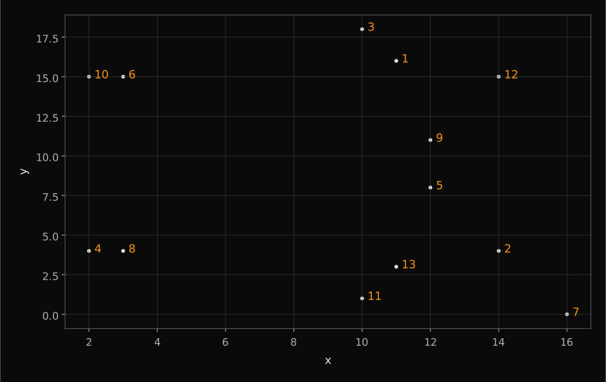
Similarly to how we could add a point to itself any number of times for elliptic curves over real numbers we can do the same for points on an elliptic curve over finite fields. Using the same point P with the coordinates (11, 16) that we used above we can “point multiply” the point to itself many times. The below plot shows all the points we end up with and how many times we point multiplied the point (1 = P, 2 = P + P, 3 = P + P + P, …):

The 13 non-identity multiples of P = (11, 16); 14P is infinity.

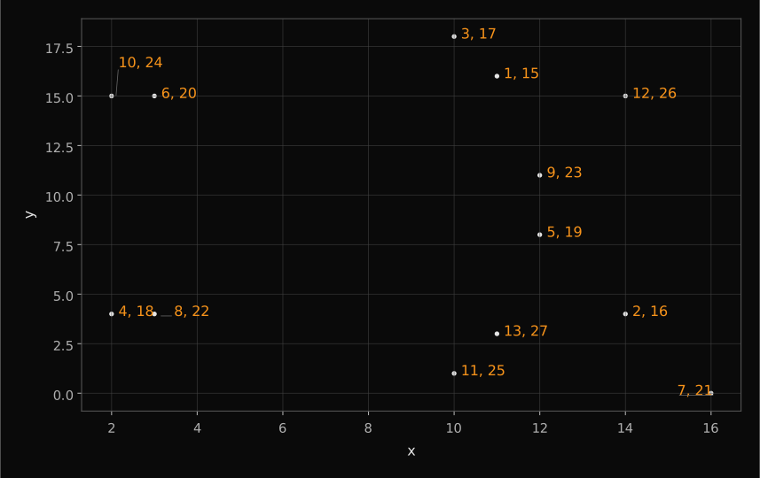
The heighest multiple of the point that you see above is 13. What if we want to add the point P to itself more than 12 times (i.e. point multiply more than 13 times)? We get the following:

The subgroup repeats every 14 multiples, with nP = (n + 14)P.

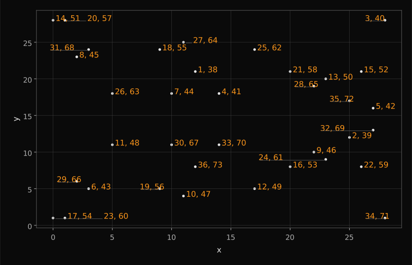
Note that the points we end up with are still all the same but now we labelled them with two values. Both of these are valid numbers for how many times we point multiplied the point, i.e. they are all valid values for nP.

Two important observations:

There is no n = 14 in the labels.

All the labels have a number n and then another number n+14.

This is due to the fact that each point on the elliptic curve over a finite field has an order. The order of a point P on the curve is defined as the samllest integer, n such that nP = O (where O is the point at infinity). In the example above, the point P therefore has the order 14. The set of points we can generate using the point P is called a cyclic subgroup of the group of points on the curve.

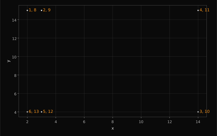
If we choose another point on the curve, (2,15), for example, we get the following cyclical subgroup:

The cyclic subgroup generated by (2, 15) on y² = x³ + 8 modulo 19.

The above plots demonstrate what happens when we point multiply points on an elliptic curve that have an order that is less than the order of the group of all points on the curve: the point multiplication results in a subgroup of points, often with way less points than all possible points on the curve. This tends to happen when the order of the group of all points is not prime (In the above example the full group has order 28: 27 affine points plus the point at infinity).

In elliptic curve cryptography we use a generator point of a large prime-order subgroup. Its order n divides the full group order N, so N = h⋅n, where h is the cofactor. The generator need not generate every point on the curve; for Bitcoin’s secp256k1, h = 1, so it does.

The reason why we need such a generator point will become clear once we talk about public and private keys.

Generator point with prime order

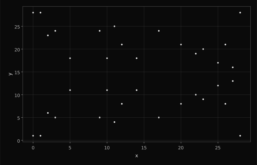
Let’s look at the set of points that fall on the elliptic curve y² = x³ + 28x + 1 over the finite field F₂₉:

The 36 affine points of y² = x³ − x + 1 modulo 29; including infinity the group order is 37.

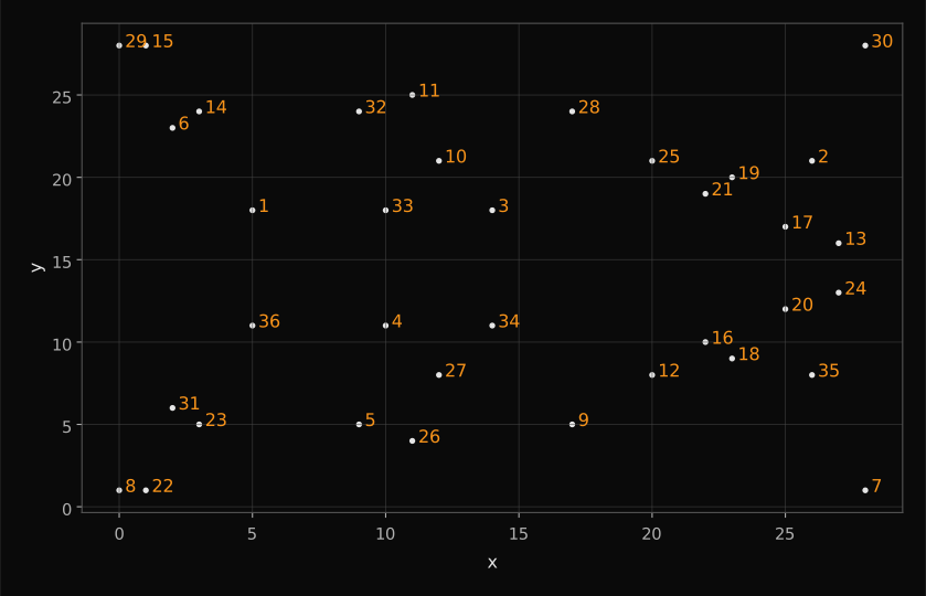
The order of the group of points that fall on this “curve” is 37. Let’s pick one of the points, (5,18), and see what the multiples of point multiplying it look like:

The generator (5, 18) reaches all 36 non-identity points modulo 29.

We can see that the point (5,18) is able to generate all other points on the elliptic curve by adding that point to itself repeatedy. The order of the generator point is 37, which is also the order of the full group and is a prime number. In fact, any non-identity point (points that aren’t the point at infinity) could be used as a generator point in this case because all of them are able to represent all other points through point multiplication. Therefore, any of these points would be a good generator point for ECC (although we would need a finite field with a much larger prime order!).

If we add P to itself more than its order, n, times, we get the cyclical group pattern again:

The order-37 subgroup repeats after 37 multiples of the generator.

Why the order and generator point matter so much

One of the key reasons why we use a generator point P of large prime order n is that we have the following:

For any integer k in the range [0, n−1], kP will be a unique point. This means that as long as k is smaller than the generator order, point multiplying the generator point by that k will lead to a point on the curve that is unique and therefore there is a one-to-one mapping between valid integers k and resulting point kP. If k was allowed to be greater than or equal to n, this one-to-one relationship wouldn’t hold anymore because of the cyclical nature of the group.

Furthermore, choosing k uniformly from 0 to n−1 gives a uniform distribution over the subgroup generated by P. Given k and P, anyone can efficiently compute Q = kP. The hard problem is the reverse: recovering k from P and Q.

For elliptic curve cryptography, especially the creation of private and public keys these properties are of extreme importance. We will dive further into this when we look at Bitcoin’s elliptic curve as well as private and public keys.

Elliptic Curve Discrete Logarithm Problem (ECDLP)

Looking at the above plots, the points seem to jump around almost randomly. Recovering the multiplier from the starting and final points is the discrete logarithm problem. Trying every integer is one approach, but generic classical attacks such as Pollard’s rho algorithm need roughly √n group operations rather than n, where n is the subgroup order.

This is the essence of the ECDLP, which states:

Given a point P and a multiple of it Q = kP , where k is a secret integer, the challenge is to find k. Despite knowing both P and Q, computing k is believed to be computationally infeasible for a securely chosen curve and a sufficiently large prime-order subgroup. This is what makes elliptic curve cryptography secure.

Why use elliptic curves over finite fields and not over real numbers

One might wonder why we use elliptic curves over finite fields and not over real numbers. What’s the added benefit of this? The key reasons are the following:

Discrete and Predictable: Over real numbers, operations like point addition and multiplication can lead to points with coordinates that are irrational or require infinite precision to represent accurately. This complicates the computation and storage of points.
Efficiency of Computations: Computations in finite fields are much more efficient. Operations like addition, multiplication, and especially division (inversion) in finite fields can be performed using modular arithmetic, which is computationally less intensive than dealing with the continuous and potentially infinite precision of real numbers. This efficiency is crucial for systems like Bitcoin where speed in transaction verification is important.
Security: Security depends on the curve and its subgroup order, not just the field size. For secp256k1, an order close to 2²⁵⁶ gives roughly 128 bits of classical security against generic discrete-logarithm attacks.
Uniform Distribution: A uniformly chosen scalar modulo the generator’s order gives a uniformly distributed point in its subgroup.
Deterministic Operations: Using finite fields makes the operations on elliptic curves deterministic and repeatable, which is crucial for cryptographic protocols.

Now that we understand how elliptic curves over fintie fields work as well as what a generator point is and why it’s important we can finally move on to Elliptic Curve Cryptography, the magic behind Bitcoin’s security. Enjoy!

Bitcoin’s Cryptography Explained — Bitcoin’s Curve

The Ellitptic Curve of Bitcoin

Bitcoin’s Cryptography Explained — Part III of V

← Part IIBitcoin’s Cryptography Explained — Elliptic Curves

Part IV →Bitcoin’s Cryptography Explained — Bitcoin’s Curve